
Executive summary
In this blog post, we present the results of our comparative 12-hour benchmark of Aerospike 3.8.2.3 vs Apache Cassandra 3.5.0 using a mixed read/write workload typical of modern internet applications. The benchmark uses YCSB (Yahoo! Cloud Serving Benchmark) and contains detailed guidelines to reproduce the results.
The benchmark shows that Aerospike provided 14x the throughput of Cassandra while also delivering 42x lower read latency and 24x lower update latency (95th percentile).
The impact of the increase in performance is fewer servers than Cassandra – and thus lower hardware and maintenance costs – for a given project. A similarly sized Aerospike cluster can absorb 14x more requests before you need to add more servers, or dramatically reduce your infrastructure footprint on day one.
Introduction
While there are many benchmarks for operational and NoSQL databases, the vast majority are for short test periods, normally less than an hour. In the Aerospike Database Manifesto, we point out the problems of short-term small tests, and propose that benchmarks should be done over an extended period of time. We performed a benchmark test to compare Aerospike’s open source project vs. Apache Cassandra’s, with a 12-hour test period. We tested with data center class servers with Intel Xeon processors, 32 GB of RAM, Intel S3700 SSDs, and 10GbE networking.
All databases have periodic background tasks that are essential for the long-term health of the database; however, these take up resources, and thus, reduce performance. By carefully tuning these background tasks – or disabling them – you can achieve remarkable but unsustainable results. We decided to run each database for 12 hours using configuration guides published by Aerospike and Datastax, one of the commercial Apache Cassandra vendors.
Most importantly, we have provided in excruciating detail instructions on how to reproduce these results. These guides include the installation and configuration of Aerospike, Cassandra and YCSB. Our goal is to make it possible for everyone to easily reproduce this benchmark, but more importantly, to allow you to critique our tuning parameters, easily try your own workloads, and generate results for different hardware.
The results are compelling. If you look at the high-level charts, you will see that Aerospike showed more than 14x the throughput of Cassandra (Figure 1), as well as 95th percentile read latencies that were 42x lower than Cassandra’s, and update latencies that were 24x lower (Figure 2) than Cassandra’s.
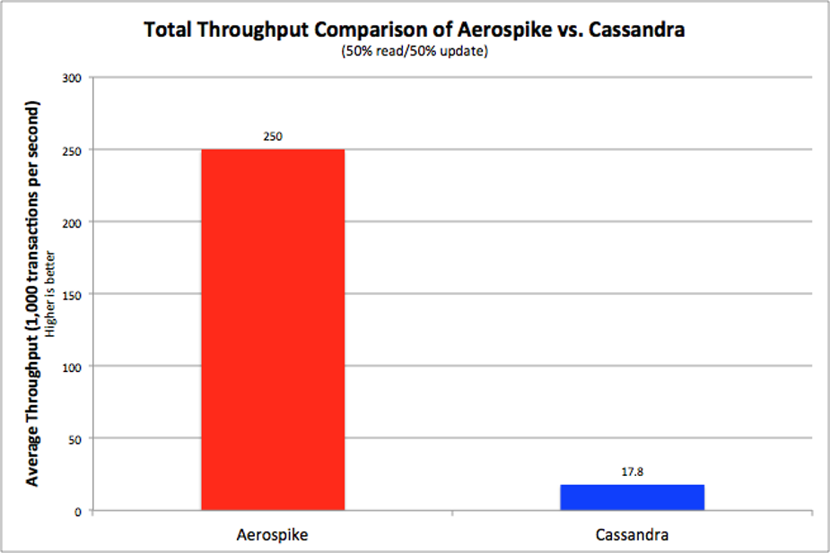
Figure 1. Throughput Comparison (higher is better)
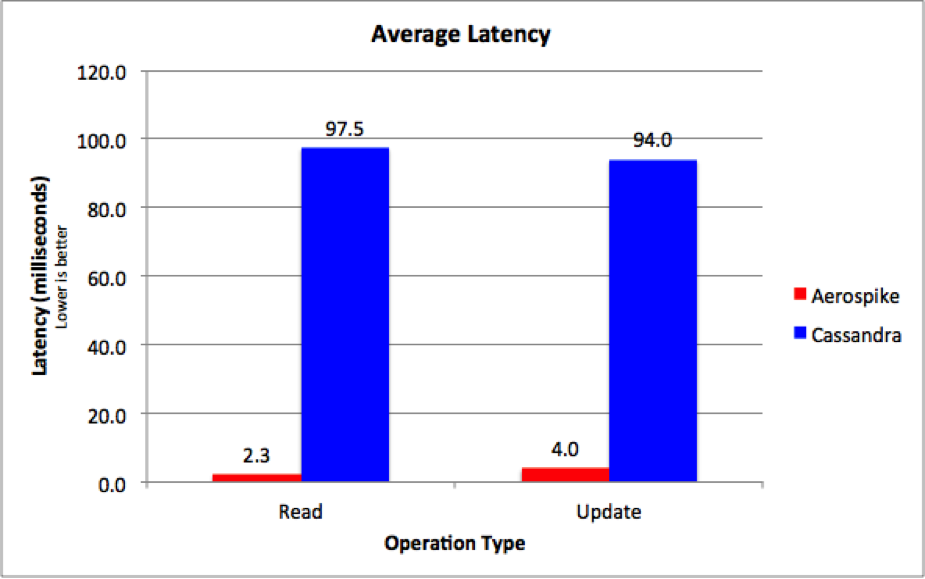
Figure 2. 95th Percentile Latency Comparison (lower is better)
As you will see in subsequent sections, it’s not just throughput and latency where Aerospike shows significant gains – it’s also the variance. Aerospike’s results have significantly more predictable response times for requests – a crucial characteristic for application developers and operation teams.
The Yahoo! Cloud Serving Benchmark (YCSB)
The Yahoo! Cloud Serving Benchmark (YCSB), originally developed by Yahoo!, is a well-known and respected benchmark tool often used to compare the relative performance of NoSQL databases. There have been many community contributions to extend its functionality, the workloads it can run, and the vendor products it can support.
Both Cassandra and Aerospike provide functionality well-suited to the YCSB benchmark, which simulates typical workloads you would find in Internet-type deployments. The benchmark is broken into two phases; data load and workload execution. For both, YCSB measures throughput, latency, and other statistics. The measurements form the basis of the results presented in this paper.
To ensure a fair comparison, we gathered the results after setting up each product using the vendor’s best practices, using the same hardware, and measuring multiple executions of the workloads, each for a minimum of 12 hours.
How we chose to configure YCSB
We chose to use the uniform distribution (the default) over the Zipfian distribution for YCSB, as the former covers the case of a highly diverse read/write workload. Further, Zipfian distributions hide the performance characteristics of the underlying infrastructure, as a significant percent of operations – often 80% – are served from DRAM cache rather than from storage. By contrast, uniform distributions cause a much higher percentage of operations to access storage; any inefficiencies in the code stack or layers of an architecture are more clearly exposed. So essentially, the uniform distribution magnifies any inefficiencies.
Since effective use of storage is a key part of an efficient system, we configured YCSB to ensure that there was more data than would fit purely in DRAM. This ensured that storage became a key measurement of the efficiency of the system.
Finally, we chose a mixed 50/50 read/write workload to show any inefficiencies in locking, concurrency, and parallelism, as both reads and writes are executed to the same data store.
We ran the tests continuously for 12 hours. Our goal was not just to understand initial peak performance, but rather, to comprehend the performance of the system over time as various periodic management processes ran, such as defragmentation of disk, garbage collection, and compaction. Indeed, these processes could affect overall throughput and latency of operations. We added the ability to record a histogram of transaction latency to YCSB, since average or total latency is a poor metric, as it doesn’t show time granularity. We’ve included this metric in our fork of YCSB, and have submitted Pull Request #753 to the official YCSB repository, as we believe YCSB discussions will be greatly enhanced by a detailed understanding of latency.
We’ve detailed our configuration of YCSB – and how we ran it – on the web page titled “Recreating the Benchmark – Aerospike vs Cassandra: Benchmarking for Real”.
Amount of DRAM per server
We agonized over how much DRAM to use per server. Between exploring all the Cassandra tuning parameters and the myriad of possible hardware configurations, we were unsure where to start with DRAM density. The Cassandra Hardware page of the Cassandra Wiki recommends “at least” 8-16 GB per server. The Datastax Cassandra Planning pages recommend from 16-64 GB (32 GB is directly in the middle), but caution that read performance will improve with larger DRAM footprints because of the effect of caching – specifically, the row cache. All in all, we believe that 32 GB footprint is a reasonable starting point.
Important note – Tests do not include major compactions
While in all our tests, we made every attempt to use the same hardware and settings to the best of our ability, there was an important difference that it was not possible to fully reconcile: major compactions for Cassandra, which, if included, would further reduce Cassandra’s overall performance.
Much of the work in tuning Cassandra involved configuring minor compactions. As these occur frequently (every few minutes), they necessarily happen during a 12-hour test. However, to perform a test that was truly fair, we would have needed to take into account the impact of major compactions, which are often scheduled weekly. For practical reasons, we did not include major compactions in these results. Doing so would have further penalized the throughput and latency of Cassandra.
Aerospike has no concept of major or minor compactions. It handles the functionality of compaction using jobs called defragmentation; these ran continuously during the test.
Methodology
In order to properly test the use case, we separated the benchmark process into several distinct phases:
Define data and test parameters, namely:
400M unique records
10 fields of 100 bytes each (total of 1,000 bytes) per record
Replication factor of 2
Strong consistency
Determine hardware based on the test parameters
Load supporting monitoring tools and applications (e.g., NTP, iostat, dstat, htop).
Install and configure a 3-node cluster with recommended settings. Verify the cluster is operating normally.
Configure each database to get the best performance with the given hardware. Run short test runs (10 minutes) to validate changes in configuration. See the references below for the recommended settings:
Load data set of 400 M records.
Cassandra only: wait for any compactions to finish in order to obtain a known starting state for the test. The time to let compactions finish (72 minutes) significantly increased the total preparation time for the benchmark tests, from 2 hours 48 minutes to 4 hours.
Clear the OS filesystem cache (for Cassandra only, as Aerospike does not use a filesystem).
Run tests for 12 hours.
Collect data, generate graphs, and analyze results.
Repeat steps 5-9 for each database.
Test results
Results summary
The raw numbers for the test results are striking. Table 1 summarizes the high-level results and the ratio of values.
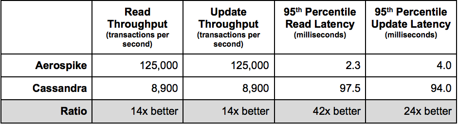
Table 1. Summary of Results
The final row of Table 1 shows the relative performance of Aerospike vs. Cassandra. This demonstrates the clear performance advantage of Aerospike.
Load time (Insert rate)
During our testing, we observed significantly different load times for Aerospike vs. Cassandra. We therefore wanted to track the total amount of prep time for each database prior to running the benchmark. Our findings are summarized in Table 2 and Figure 3 below:
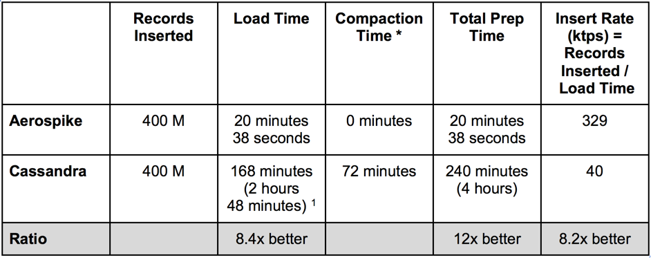
Table 2. Insert Rate
The insert rate of Aerospike was measured at 8x that of Cassandra. We took this measurement during YCSB’s load phase, which is not included as part of the workload phase and simulates a 100% write workload. When you take compaction into account, the performance difference between the two databases is even more striking as it increases to 12x. Cassandra is known for its ability to process inserts, but as shown above, Aerospike is able to load the same data set significantly faster and without the need for a settling period to allow compactions to stabilize.
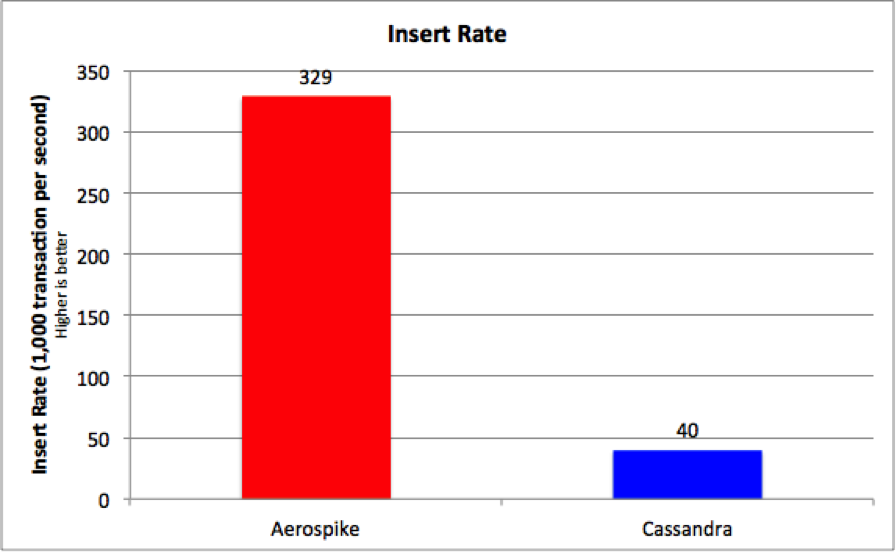
Figure 3. Insert Rate Comparison (higher is better)
Read results: Throughput and latency
Mixed reads and writes are applied during the workload phase. Our test results show that Aerospike has, on average, 14x higher read throughput than Cassandra on the same hardware (see Figure 4 below). Note that the variance in the throughput is negligible for Aerospike (red line) but significant for Cassandra (blue line).
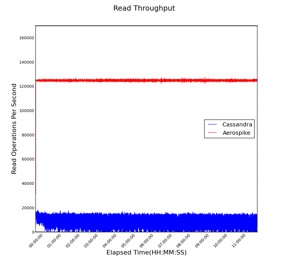
Figure 4. Read Throughput (higher is better)
While throughput with Aerospike was higher, latency was lower. In most operational use cases, predictable read latency is critical. Figure 5 (below) shows the 95th percentile of latency; critically, Aerospike has 42x lower latency with very predictable and low variance response times, as can be seen by the very narrow band (in red).
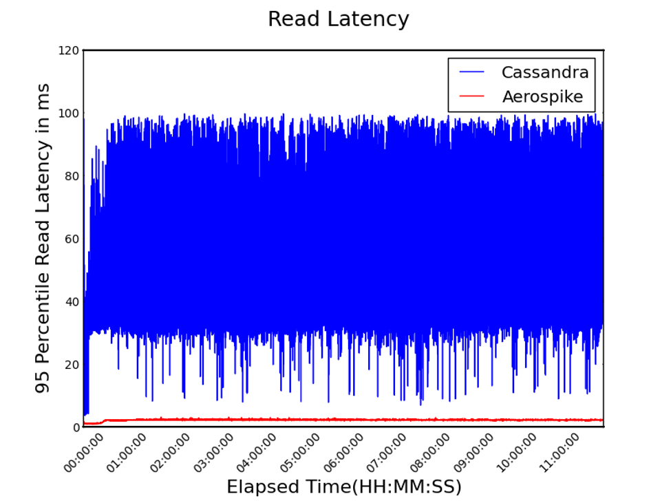
Figure 5. 95th Percentile Read Latency (lower is better)
In contrast, Cassandra has not only 42x higher latency, but most significantly, a wide variance between the slowest and fastest response times (in blue), leading to very unpredictable response time for your application.
Within the first half-hour, latencies change. For Aerospike, this increase is caused by a background process called “defragmentation.” Defragmentation is database garbage collection on the SSD. It is not clear to us what causes this increase for Cassandra, but it is most likely a background process such as compaction.
Update results: Throughput and latency
With a read / write mixed workload, we can also examine the performance of updates. Any underlying contention between reads and writes will manifest as lower throughput and higher latency. Aerospike achieved a 14x improvement in average throughput (Figure 6) and 24x lower latency (Figure 7), showing the effectiveness of its implementation.
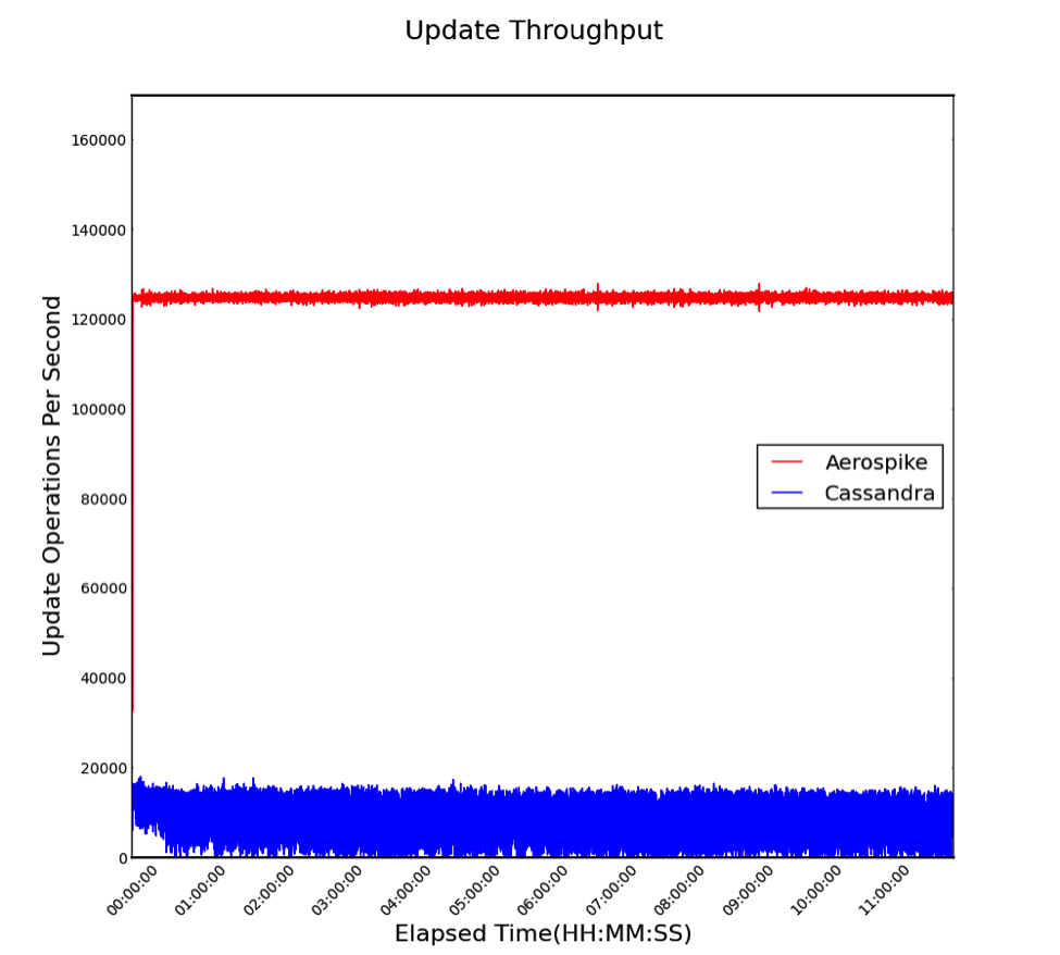
Figure 6. Update Throughput (higher is better)
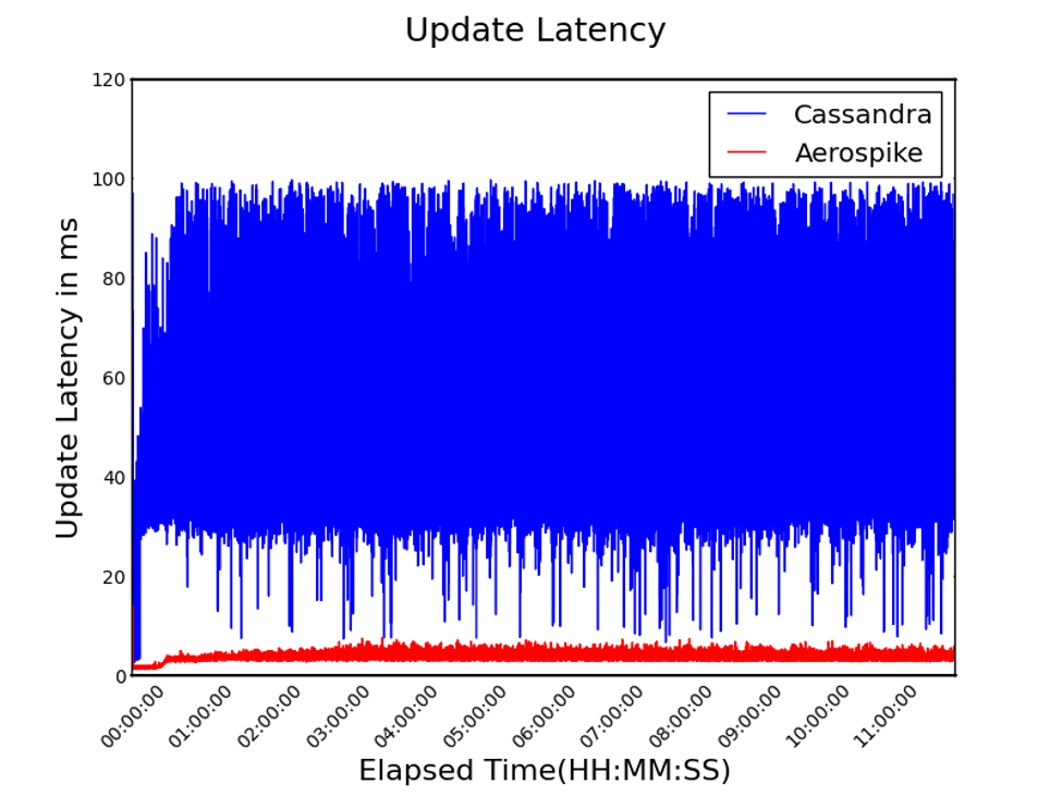
Figure 7. 95th Percentile Update Latency (lower is better)
The 95th-percentile update latency chart (see Figure 7 above) shows that Cassandra (in blue) has much greater variance in update latency, which translates into inconsistent response times. As was seen in the Read Latency graphs, there is a change approximately a half-hour into the run as the various systems processes (e.g., compactions, defragmentation) start to impact the system. By comparison, Aerospike (in red) shows minimal variance; thus, Aerospike’s response times make it far more predictable than Cassandra.
Conclusion
Our testing shows that over extended mixed workloads tests, Aerospike simultaneously delivers vs. Cassandra:
14x greater throughput than Cassandra
42x lower read latency than Cassandra
24x lower update latency than Cassandra
8x greater insert throughput than Cassandra
We believe these findings are significant, given the perception that Cassandra is designed for high-volume and low-latency operations against datasets larger than DRAM. Aerospike delivers much higher performance than Cassandra with significantly lower variance, meaning its performance is very predictable, with low jitter.
For the IT or Line of Business budget, this means the following:
Aerospike can accommodate your future growth at a lower cost
A similarly sized Aerospike cluster can process 14x more transactions, with
42x lower query latency and
24x lower update latency
Aerospike shows significantly reduced TCO (Total Cost of Ownership)
Choosing Aerospike could reduce your cluster size 14x on day one
Aerospike provides predictable performance
Aerospike lets you reduce the complexity of operationalizing your applications
We encourage you to run this benchmark on your infrastructure for your particular workload, and examine the results for both Aerospike and Cassandra. Making full use of the performance and latency advantages of Aerospike provides a cost-effective way to drive your business.
In order to stave off controversy and make it possible for you to recreate our benchmark, we have provided extensive detail about our benchmark settings, as well as copious instructions on how to run the tests. We welcome an open discussion of our findings. If you’d like to voice any thoughts or observations about the benchmark, or share your own experience about using Aerospike or Cassandra in production, please do so on our user forum. We look forward to the dialog.
If you would like to try this benchmark for yourself, please go to the web page titled “Recreating the Benchmark – Aerospike vs Cassandra: Benchmarking for Real”.
If you would like to request a free Aerospike Enterprise Trial, please contact us.
Software and hardware for benchmark
Software
In our testing, we compared the open source versions of both Aerospike and Cassandra. We decided to use recent builds of Aerospike (Community Edition version 3.8.2.3) and of Apache Cassandra (version 3.5.0). The OS distribution used was Centos 6.7, and the Java version was Oracle Java Hotspot 8.0.60.
Hardware
The hardware we chose reflects what you would typically see in a data center today. This allows anybody to reproduce these results without needing the latest and greatest hardware. As Aerospike and Cassandra are different databases with very different requirements, we selected hardware that works equally well for both databases:
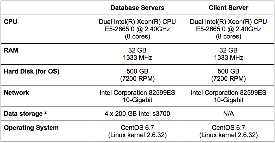
Table 3. Hardware Selected for Our Benchmark
Appendix A – Notes from cassandra testing
Basic installation and hardware choice
We had a very large number of options to consider – and thus, many choices to make – when deciding how to configure and install Cassandra. Our goal was to run a fair and reasonable benchmark based on what we learned from the most highly regarded experts in Cassandra.
We decided to use the open source version of Apache Cassandra for our benchmark. The 3.5.0 version was released April 13 2016, and we used the binary version from Apache’s website. As there is no package (a common occurrence for Java-based Apache projects), we simply decompressed the distributed binary image into a directory.
While many Cassandra installations use SSDs, there isn’t a large body of information about how to configure for SSDs. There are several recommended parameter changes to optimize for SSDs, but a key question remained: which filesystem to use. We primarily followed the recommendations from Datastax, who provides support for Apache Cassandra and can be regarded as experts in the field, but Datastax makes no recommendation on file system. We then took advice from the recommendations of Al Tobey, who strongly recommends XFS. We formatted each SSD with the XFS file system and added each as a separate data directory in the Cassandra config file.
We also needed to increase the default system file handle limit. Without this limit increase, the initial long duration tests would have run out of file handles, and Cassandra would have halted instead of continuing to run with warnings. Here again, we modified the settings in sysctl and limits.conf using Al Tobey’s recommendations.
In order to create a standardized benchmark, Cassandra must be allowed to finish compaction after data loading. We monitored the amount of compaction, and only started the benchmark after Cassandra’s compactions had ended.
Tuning parameters
Tuning compaction throughput. During the early runs of the benchmark, Cassandra fell way behind in compactions, and eventually slowed to a crawl or crashed. Why is that? The default value of 16 MB of compaction per second in Cassandra doesn’t work well for benchmarking and for stress-testing the database. As we attempted to try different settings with throttled compaction, we found that eventually, the compaction rate could not keep up with the constant load over 12 hours. Many people have noted (e.g., Ryan Svihla in “How I Tune Cassandra Compaction”) that compaction should be tuned so that it can catch up during lower traffic times.
However, since we were attempting to find the maximum level of constant traffic, there would be no period of lower traffic. We suggest that it is always good to estimate the maximum sustainable level of traffic, since once you hit that level, compaction will not keep up. In the end, we found that disabling compaction throttling led to the highest continual throughput for the 12-hour duration.
Tuning the row cache. We had to decide whether to enable the row cache, and if so, what values to use in order to configure it correctly for our workload. The row cache is only recommended if you can achieve a high hit ratio; otherwise, the row cache decreases performance. In our estimation, this workload – which with a uniform distribution, does not have a large percent of cache hits – does not benefit from the row cache. With the estimated data size, the row cache would have to be around 120 GB per node, but each of the nodes were configured with 32 GB of memory. Thus, we disabled row caching.
Tuning the key cache & JVM heap size. We had trouble finding sensible guidelines on optimizing the key cache. Datastax recommends a JVM heap size of ¼ of DRAM up to 8 GB, which we used. For a uniform workload, achieving a Datastax-recommended optimum hit ratio of 95% would require more than 11 GB of RAM per machine for key cache – far exceeding the 8 GB of the JVM heap – so reaching an optimal key cache size was not possible. After some experimentation, we found that larger key cache sizes increased latency. Thus, we set the key cache size to 1 GB.
Tuning the Java garbage collector. Much has been written about which garbage collector to run with which Cassandra workloads. We tried both the CMS and G1GC garbage collectors. The overall performance did not seem to vary greatly between the two, but since we wanted to configure for the most common recommendations, we ended up choosing the G1GC (the G1 Garbage Collector) for the longer runs.
Datastax suggests G1GC for heaps larger than 4 GB. Below are some supporting documents for the choice of garbage collector:
https://www.infoq.com/articles/Make-G1-Default-Garbage-Collector-in-Java-9
https://sematext.com/blog/2013/06/24/g1-cms-java-garbage-collector/
Choosing the compaction type. There are two options for compaction: size-tiered, and leveled. Size-tiered compaction is recommended for write-heavy workloads. Leveled compaction is recommended for read-heavy and update workloads. As our benchmark uses ‘YCSB workloada’, which specifies a balanced load of 50% reads and 50% writes, we selected leveled compaction. The following links from Datastax provide the reasons for using leveled compaction:
http://www.datastax.com/dev/blog/leveled-compaction-in-apache-cassandra
http://www.datastax.com/dev/blog/when-to-use-leveled-compaction
Tuning the read and write threads. We looked at recommendations for both of these parameters. Datastax recommends that the number of write threads should be increased in order to be identical to the number of cores in the system. The default number of read threads also follows Datastax’ recommendations, and seemed to provide a reasonable level of performance.
Tuning the commit log. We left the commit log on for durability of writes, which matches the characteristics of Aerospike. In our test, turning off the commit log made little visible difference to the results we measured.
Client tuning
In order to create a consistent test environment, we started with a relatively small number of threads and continued to increase the number of threads until throughput topped off. While Aerospike was able to handle up to 1,500 client threads, Cassandra could not complete testing at that level. We eventually settled on 800 client threads as a good level for which both databases could complete the 12-hour test.
Consistency
Cassandra has configurable consistency. We selected a consistency level of 2 for writes and 2 for reads to make the test comparable. This consistency level removes the “dirty read problem” where an application may read stale data after a write; it’s comparable to Aerospike’s default consistency mode. A small test was run to see the difference between a consistency level of 2 vs. 1. The difference was about 2,000 operations per second. This difference is not large when comparing Aerospike vs. Cassandra.
Appendix B – Notes from Aerospike testing
Although we’re experts at using Aerospike, for the lay user, Aerospike provides a number of features to make installation simpler. For instance, Aerospike distributes standard Linux packages for easier installation and version management. Moreover, Aerospike is installed as a service.
Aerospike uses only one file for configuration, which defines the DRAM and storage devices, the number of threads, as well as the other nodes in the cluster. The number of threads needs to be set, as well as the amount of memory to be allocated. We followed Guidelines from Aerospike for service-threads to set these parameters, which depend on the hardware.
Aerospike handles the the equivalent of Cassandra compactions with defragmentations. These are run continuously, but with short sleep pauses in between. For systems that will be under high write stress, like this benchmark, the recommendation is to set defragmentation sleep time to zero. Please see the Aerospike page on storage for more info.
Aerospike uses raw devices, so there is no need to pick a file system (e.g., XFS, EXT4, etc.), and the database does not have a separate commit log. This simplicity makes hardware planning easier, as well as configuration.
Footnotes
Cassandra’s load time included only the actual inserts. Prior to beginning the benchmark tests, we waited an additional 72 minutes to let compactions complete in Cassandra. We did this in order to create a reliable starting point for testing. Since Aerospike handles the equivalent of compactions differently, it does not require a waiting period before testing can begin.
The motherboard’s hard disk controllers went through a lower-end RAID controller; this added a little latency to query times. The SSDs were not placed into a RAID array, but there was an impact on latency. As a result, the SSDs here do not perform as well as they could have if they’d simply been attached to the motherboard or on a higher-end RAID controller. Both Cassandra and Aerospike used this same setup.
Keep reading

Jun 17, 2026
Fail fast, stay resilient: How to stop hidden gray failures in Aerospike on AWS EBS

May 28, 2026
Determining the best machine learning and AI databases

May 18, 2026
The three price tags: How Redis unpredictability costs you infrastructure, engineering time, and UX

May 12, 2026
Monitoring Aerospike Enterprise in Datadog: What you get and how it works