
Prior to Aerospike v3.9.1, we defined the maximum cluster size using a config parameter. Cluster size defaulted to 32, with a maximum value of 128:
service {
        paxos-max-cluster-size 32
}
Once the cluster was established, it could then grow to the value specified by this parameter. This meant that:
Nodes could be dynamically added, up to the value of paxos-max-cluster-size
Additional requests to join the cluster were rejected
paxos-max-cluster-size could only be changed by a cold cluster restart
Therefore, without planning, you could reach a point where you had no option other than doing a cold cluster restart in order to expand the size of the cluster. This is a poor operational model. Typically, you’d want this value to be right-sized, as it governs the size of of various data structures that are transmitted over the wire.
Heartbeat Algorithm v3
Starting in Aerospike v3.9.2, we’re introducing a revision of the Heartbeat algorithm – v3. The goal of the project is to:
Simplify the operational experience
Allow dynamically adding nodes, up to the maximum cluster size allowed by the edition
Allow clusters to transition from Community to Enterprise Editions
Operationally, there are two aspects to cluster formation:
Speed of cluster formation
Stability of the formed cluster
No single aspect above dominates the decision-making. Both are important in certain situations. When the network is stable, we give higher importance to the speed of cluster formation; and when it’s unstable, we give higher importance to cluster stability.
In the old algorithm (v2), especially with the mesh mode of clustering, we used to go through multiple rounds of cluster formation before we discovered all nodes and reached a fully formed, stable cluster. In the old algorithm, we used to exchange only the information about the well-formed cluster. In the new algorithm (v3), however, we exchange information not just on the state of the cluster, but also on the nodes that are visible, but not yet part of the cluster. With this extra information, all the nodes discover each other more quickly, and form a cluster faster and more accurately.
For example, let us consider 3 nodes – N1, N2, and N3. In the mesh configuration, let’s say that everyone points to N1, and that N3 is going to be the principal node of the final cluster. The principal node is responsible for making sure that all nodes agree on a consistent state of the cluster. Typically, this is the node with the highest ID number in the cluster. A simplified series of events in the old algorithm (v2) is shown in Figure-1. The messages include the cluster list.
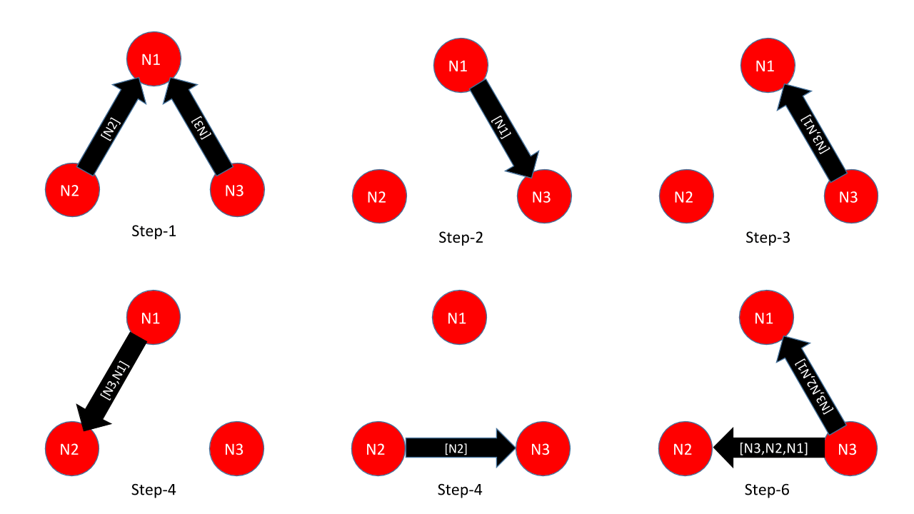
Figure-1: Cluster formation with the v2 algorithm
The steps illustrated in Figure 1 are as follows
N2 and N3 send themselves in list to N1; N1 discovers them
N1 sends succession list to newly discovered N3 (the same event is sent to N2, but we did not illustrate this to simplify the diagram)
N3 becomes the principal node among N3 and N1, and sends the cluster list to N1
N1 sends the list to already discovered N2
N2 sends succession list to newly discovered N3
N3 discovers N2 and becomes the principal node among N1, N2, and N3
In the new algorithm (v3), node discovery occurs much faster, as we not only send the cluster list (called succession list), but also the list of discovered nodes (called adjacency list). The steps are shown in Figure-2; for brevity’s sake, however, we chose to only show the adjacency list.
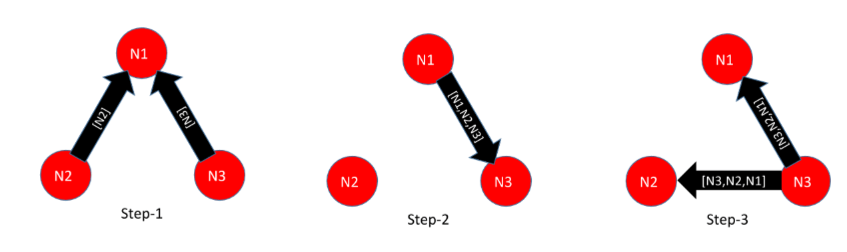
Figure-2: Cluster formation with the v3 algorithm
The steps illustrated in Figure-2 are as follows:
N2 and N3 send themselves in list to N1; N1 discovers them
N1 sends adjacency list N1, N2, and N3 to newly discovered node N3 (and also N2)
N3 discovers N2 and starts sending the full list to N1 and N2
Ironically, even though we used to exchange less information per message, overall, we ended up using a lot of messages due to the multiple rounds of cluster transformation before a steady state was reached. In the new algorithm, even though we send more information per message, we converge faster, and with fewer messages. We reduced bandwidth and connections, as well as cases with multiple connections between the same nodes, so that redundant messages to all connections no longer need to be sent.
To improve the stability of the cluster, we reduced the number of variables involved in the decision-making process. This process is mainly based on the experience we gained from the old protocol. We now avoid redundant initiating heartbeats on inter-cluster fabric messages, and buffer events to process in batches. All these improvements make forming stable clusters simpler, even in the most challenging and flaky of network stacks.
Benefits of the Heartbeat Algorithm v3
The new heartbeat algorithm has a myriad of benefits, including:
Lower consumption of network bandwidth
Compression of heartbeat data on the wire
Faster cluster formation in mesh mode, with fewer cluster transitions
The ability to have larger clusters with mesh mode
The ability to stop and restart the heartbeat layer, both in mesh and multicast mode. This also allows increasing max cluster size dynamically in mesh mode.
The introduction of cluster-name option in the service section. The heartbeat subsystem will not allow nodes with different cluster names to be in the adjacency list. This option will be dynamic, which will:
Provide an easier way to demarcate clusters
Allow very easy removal of nodes from a cluster (e.g., for re-purposing), without running tip-clear on all nodes.
Allowing DNS names (in addition to IP addresses) as seed identifiers
Other Changes
paxos-recovery-policies We removed the following paxos-recovery-policies (using these in config will generate a warning):
auto-dun-all
auto-dun-master
manual
We also restricted the port numbers to be >= 1024 and <= 65535, to be consistent with fabric
Impact to the Community Edition
With these changes, we have made the decision to limit the Community Edition to a maximum of 32 nodes. We thought long and hard about this; our conclusion was that as your cluster size grows, you increasingly need the additional features of the Enterprise Edition – such as Fast Restart and Rapid Migration – in order to effectively use wider clusters in Production. In our testing, that cut-over point was around 32 nodes.
Upgrading to the Enterprise Edition is simple, since you can run mixed Community and Enterprise editions in a single cluster. You will just need to perform a rolling restart of the existing nodes in the cluster, which can be done without taking an outage for the cluster.
Summary
As our community and our customers grow their clusters, these changes will make their Operational Experience (OX) simpler; they will also be able to use their network more efficiently. The ability to form clusters in both the Community and the Enterprise edition will allow users and customers to easily migrate to the Enterprise Edition and take advantage of its features when they need to, with no downtime.